A Matlab code for front tracking

This site will look much better in a browser that supports web standards. Your browser does not support web standards, use pgDown/pgUp to navigate.

You can download all files mentioned below by clicking on MatlabCode.zip

The front-tracking code described in the book resides in several files containing many Matlab routines. These routines perform the bookeeping needed to do the tracking. In other words, the fronts and the collision times are recorded, and the approximate Riemann solver is called, and the result inserted in the correct place. The routine that does this is called genFrontTrac and resides in the file genFrontTrack.m. The syntax for using this function is

[u,x]=genFrontTrack(u0,x0,T,delta,varargin);

Here u0 is a vector containing the initial values as a step function, of size [nc,N], where nc is the number of components, and N is the number of values. The "steps" are located at x0, which is a vector of size N-1. The variable T denotes the time at which the solution is wanted, delta is the parameter giving the accuracy of the approximate Riemann solver. The parameter varargin may contain various options, typically a codeword possibly followed by a value for that option. These must be:

'display':followed by either 'lines'; for drawing the fronts as lines, or 'polygons';for drawing colored polygons, or 'plain'; for no graphical output (default).

'save', which creates Matlab graphics that can be saved from Matlab, default not, this uses a lot of Matlab's memory. This has no value, i.e., must not be followed by any option.

'colors' must be followed by a Matlab colormap to be used for colored polygons. This option has no effect if the 'polygons' option is not used. The default colormap is jet.

'periodic' if periodic boundary conditions is used. This option must be followed by an interval [a,b], where a<x0(1)<x0(N-1)<b. Also the equality u0(:,1)=u0(:,length(u0)) must hold in this case.

Routines used by genFrontTrack

Apart from the approximate Riemann solver (we return to this below) genFrontTrack uses several utility routines.

initialize(u0,x0,T,delta) This routine creates the initial fronts by solving the Riemann problems defined by u0 and x0. It returns [u,s,t_coll,x], where u is the values of the step function approximation to the solution of the Riemann problems, s are the speeds of the fronts, x are the starting points of the fronts, (so the actual position will by given by x(t)=x+s*t), and t_coll is the collision times. The collision times are associated with an interval, therefore this is a vector of the same length as u, while s is associated with the fronts, and therefore these are of the same length. Note that if the length of u is M, then the length of x is M-1. This routine is in the file initialize.m.

collision_time(s,t,x,T) This routine calculates the collision time between two fronts. Here s=[s(1) s(2)], t=[t(1),t(2)], x=[x(1),x(2)] and T is the final time. Here the left (right) front has speed s(1) (s(2)), starting time t(1) (t(2)), and starting point x(1) (x(2)). This routine is in the file collision_time.m.

Graphical routines

Some routines are needed to produce the colored polygons. First there is the routine colfunc(u). This function determines which quantity, i.e., a function of u, that determine the color of the output. The relevant file is colfunc.m. To actually plot a color, we need an index into the colormap, the routine that gives this is clindex(u,pmax,pmin,NMAP). Here pmax and pmin give the interval of colfunc's that are plotted. If u gives a value that is outside this interval, the appropriate endpoint is used. NMAP is the lenght of the colormap, i.e., the colormap is a matrix of size [NMAP,3]. clindex is found in clindex.m.

 

The approximate Riemann solver

The most important routine in genFrontTrack is the Riemann solver. Herein resides all the physics & mathematics. The syntax for calling this is

[u,s]=Riemannsol(ul,ur,delta);

Here ul and ur are the left and right states, and delta controls the accuracy of the solution. The output is the speeds of the fronts resulting from the approximate solution; s, which is a vector of size ns, and the intermediate states u, is a vector of size [nc,ns-1]. Thus, if there is only one front, i.e., ns=1, then u=[]!

Demonstration solver

You are of course supposed to write your own Riemann solver to suit your own needs, but for demonstration purposes we have supplied a Riemann solver for the p-system of gas dynamics, for a gamma gas law with gamma=1. The calculation is done in Riemann coordinates, so in order to obtain the physical variables p (density) and v (velocity) you use the routines [p,v]=Riemann_to_Phys(w) and its inverse w=Phys_to_Riemann(p,v). The advantage of using Riemann coordinates is that the rarefaction curves are straight lines, and thus easy to compute. This Riemann solver is in the file Riemannsol.m, (which you should replace by your own if you wish to solve other problems). This needs the routines middle_state.m, Jack.m, dJack.m, states.m, sspeed.m, phi.m, dphi.m and rspeed.m.

Demonstration file

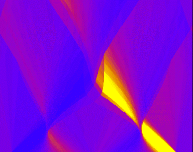
To test all this you can try to run the Matlab script ftdemo.m. This needs the utility plotFTresult.m. If you try this without any changes, you should get something like

Try out the other options, change the size of N and try other initial data, try without periodic boundary conditions, and try changing the colors. Then you are ready to write your own Riemann solver for your own problems!

Happy tracking !